Thesis: 3.2 The weighted rich-club effect

This chapter is based on an article co-authored with Vittoria Colizza, Pietro Panzarasa, and Jose J. Ramasco (see Opsahl et al., 2008).

While Eq. 6 describes whether or not ties are established among prominent nodes, it does not measure the relative strength of these ties with respect to other ties in the network. Examining the intensity and capacity of interactions is however fundamental for understanding the organising principles underpinning the structure of weighted networks.

Moreover, the prominence of a node can be defined in terms not only of its degree, but also of other properties in weighted networks. This can include the strength of the nodes (i.e., the sum of the weights attached to the ties originating from the nodes; Zlatic et al., 2008) or the average weight (i.e., the ratio between the strength and degree of the node). To determine the relative strength of the ties connecting prominent nodes, we propose the following weighted rich-club coefficient, based on a parameter r of node prominence (equation 8):

$\phi^w(r)=\frac{W_{>r}}{\sum_{l=1}^{A_{>r}}w_l^{\mathrm{rank}}}$

where the numerator is the total weight of the ties connecting the nodes that are prominent with respect to r. Given that the number of ties among the prominent nodes is $A_{>r}$ , the denominator corresponds to the sum of the weights of the $A_{>r}$ strongest ties of the network. $w_l^{\mathrm{rank}}$ is an ordered vector of all the weights in the network. This vector is ordered accordingly to $w_l^{\mathrm{rank}}\geq w_{l+1}^{\mathrm{rank}}$ and $l=1,\,2,\,...\,,\,A$ , with A being the total number of ties in the network. Thus, Eq. 8 measures the fraction of weights shared by the prominent nodes compared with the total amount they could share if they were connected through the strongest ties of the network. $\phi^w(r)$ takes values ranging from 0 to 1. It is equal to 0 if none of the ties connecting the prominent nodes are among the strongest ones, whereas it is equal to 1 when the ties connecting the prominent nodes are the strongest available ones.

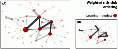
To illustrate the different elements of this coefficient, Figure 4 shows a sample network with 38 nodes out which 5 are designated as prominent ones. The prominent nodes are connected by 6 internal ties (highlighted ties in Figure 4a). Not all these 6 ties are among the 6 strongest ties in the network (highlighted ties in Figure 4b). The coefficient for this network would be the the sum of the weights attached to the internal ties (panel a) divided by the sum of the weights attached to the strongest ties (panel b).

3.2.1 Null models

In analogy with the topological rich-club coefficient, Eq. 8 might not enable us to test whether there is an actual tendency of the prominent nodes to be connected through the strongest ties in the network. This is due to the fact that some ordering properties are associated with the strength of ties. When this is the case, even random networks may display a signal. Therefore, to properly test the phenomenon, we need to assess the weighted rich-club effect observed in a real-world network against the effect found in an ensemble of random networks based on an appropriate null model. This model must generate networks that are random, but at the same time comparable to the observed network. In particular, our choice of an appropriate null model reflects the need to discount for associations between weights and ties. To this end, the ensemble of random networks produced by the null model must meet three main requirements. First, the random networks must have the same number of nodes and ties as the observed network. This ensures that the basic parameters of the networks are the same (Erdos and Renyi, 1960; Rapaport, 1953). Second, they must have the same weight distribution $P(w)$ (i.e., the probability that a given tie has weight w) as the observed network. This is a crucial constraint since we are looking for non-trivial intensity of interactions among nodes. Moreover, this guarantees that the vector of ordered weights remain the same. Third, the nodes in the selected subset (the club) must be the same as in the observed network. This preserves the distribution $P(r)$ (i.e., the probability that a given node has prominence r). A null model that does not produce an ensemble of random networks that fulfill the above three requirements cannot produce networks comparable to the observed network, and thus does not allow for a proper weighted rich-club assessment (Colizza et al., 2006).

There are multiple null models that create random networks that meet the above conditions. Nonetheless, at the same time certain models are excluded. This is the case, for example, of models in which weighted ties are considered to be multiple binary ties (e.g., a tie with a weight of 3 is considered to be 3 binary ties; Newman, 2004a; Serrano, 2008). These models do not preserve the number of ties or the weight distribution $P(w)$ of the observed network.

In what follows, we introduce three null models for constructing random networks. The appropriateness of these models depends on the choice of the prominence parameter r. If the prominence of a node is given by its degree, we adopt the following two null models. A first procedure consists simply in reshuffling the weights globally in the network (Weight reshuffle null model). This null model maintains the topology of the observed network. Therefore, the number of ties originating from a node (degree) does not change.

A second procedure, which introduces a higher degree of randomisation, consists in reshuffling also the topology, reaching the maximally random network with the same degree distribution $P(k)$ as the observed network (Maslov and Sneppen, 2002; Newman, 2003). It does so by randomly selecting two ties, $i_1 \to\hspace{-14pt}_{w_1}\hspace{+4pt} j_1$ and $i_2 \to\hspace{-14pt}_{w_2}\hspace{+4pt} j_2$ . The two ties are then rewired by setting $i_1 \to\hspace{-14pt}_{w_1}\hspace{+4pt} j_2$ and $i_2 \to\hspace{-14pt}_{w_2}\hspace{+4pt} j_1$ . The weights are automatically redistributed by remaining attached to the reshuffled ties. However, if either of these ties is already formed, this step is reverted, and two new ties are selected. This condition guarantees that multiple ties are not formed between two nodes, which ensures that the weight distribution $P(w)$ and degree distribution $P(k)$ remain unchanged. If this procedure is repeated enough times, the outcome is a corresponding random network (Weight & Tie reshuffle null model). (Since this model is commonly used in the Physics literature, we apply it here. However, each of the random networks that can be produced with this model is not produced with an equal probability of the null model. For more details, see Snijders (2001) and Rao et al. (1996).)

While both randomisation procedures preserve $P(k)$ and $P(w)$ of an observed network that can be either directed or undirected, they differ in that the Weight & Tie reshuffle alters the location of the ties, and thereby destroys node-node topological correlations. Therefore, a rich-club coefficient based on the latter null model will mix the effect coming from the location of the strongest ties and that coming from the topology. We consider it here for the sake of comparison, since it is the method used to calculate the topological rich-club effect (Colizza et al., 2006), and also to check the effect of higher degrees of randomisation on the obtained results.

Inevitably, since weights are reshuffled globally, both procedures produce random networks in which the nodes do not maintain the same strength s as in the observed network. Therefore, when prominence is based on node strength, we need to introduce a third randomisation procedure that preserves this quantity. We construct a null model based on the randomisation of directed networks (Serrano et al., 2007) that preserves not only the topology and $P(w)$ , but also the strength distribution $P(s)$ (i.e., the probability that a given node has strength s). To this end, we reshuffle weights locally for each node across its outgoing ties (Directed Weight reshuffle null model). In so doing, we also obtain null models where the average weight of outgoing ties is kept invariant. We extend this procedure to undirected networks by duplicating an undirected tie into two directed ties — one in each direction. It should be noted that this procedure breaks the weight symmetry in the two directions of an undirected tie (the topology remains invariant). The appropriateness of this method for undirected networks depends on the research setting and how tie weights are defined. For example, its applicability to undirected transportation networks is justified by the typically directed nature of traffic flows (although the US airport network displays a high symmetry; Barrat et al., 2004). Conversely, in an undirected collaboration network this might not be appropriate. In particular, for projections of two-mode networks, it might be more appropriate to reshuffle the two-mode structure before projecting it onto a one-mode network (see Rao et al., 1996; Snijders, 1991). 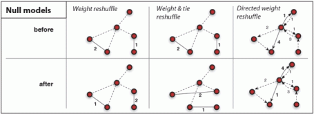Nevertheless, we choose to apply this method due to the lack of better methods and a procedure which maintains $P(s)$ and the weight symmetry would constrain the produced random networks to an extent that they would differ from the observed network only slightly. Figure 5 shows a schematic representation of the three methods.

An additional null model that reshuffle the two-mode structure before projecting it onto a one-mode network has been suggested and tested in the following post: Weighted Rich-club Effect: A more appropriate null model for scientific collaboration networks.

Figure 5: Randomisation procedures: Representation of a single reshuffle. Solid lines correspond to the ties that are randomised; the number attached to the ties refers to their weight. The Weight reshuffle procedure randomises the weights globally in the network, while keeping the topology intact. The Weight & Tie reshuffle procedure introduces a higher degree of randomisation by reshuffling also the topology, while preserving the degree of each node (Molloy and Reed, 1995; Newman and Park, 2003). Weights are automatically redistributed as they remain attached to the reshuffled ties. The Directed Weight reshuffle procedure reshuffles weights locally for each node across the ties originating from the node (Serrano et al., 2007). This figure is based on the third part of Figure 1 in Opsahl et al. (2008).

As with the topological rich-club coefficient, we define the normalised weighted rich-club coefficient as the ratio between the value obtained by Eq. 8 measured on the observed network and the value obtained on an ensemble of corresponding random networks (equation 9):

$\rho^w(r) = \frac{\phi^w(r)}{\phi_{\mathrm{null}}^w(r)}.$

When $\rho^w$ is larger than one, the observed network has a positive weighted rich-club ordering, with prominent nodes concentrating a disproportionately large part of their efforts towards other prominent nodes compared with what happens in the random null model. Conversely, if $\rho^w(r)$ is smaller than one, the ties among the prominent nodes are weaker than randomly expected.

3.2.2 Significance of effect

The randomly expected value, $\phi_{\mathrm{null}}^w(r)$ , is obtained by taking the average of $\phi^w(r)$ measured on many random networks created using an appropriate null model. Even though the random networks are based on the same null model, the values that constitute the average varies. This is because each sampled random network is different from each other. We have found that when few nodes and ties exist within the subset of prominent nodes, the values found for the random networks can differ considerably. In fact, a striking outcome of $\rho^w(r)$ might be reproduced in a large proportion of the random networks when the definition of prominence is very restrictive.

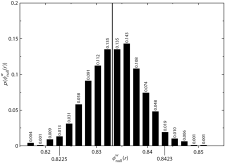
Here we analyse the variation in the values of $\phi_{\mathrm{null}}^w(r)$ . These values can be plotted as a distribution that shows the frequency of their occurrence. Figure 6 shows the distribution of $\phi_{\mathrm{null}}^w(r)$ obtained from 1,000 random networks created from the online social network (see Section 1.4) when prominence is defined as having more than 5 contacts ( $\phi^w(k>5)=0.935$ ) using the Weight reshuffling.

The values of $p(\phi_{\mathrm{null}}^w(r))$ can also been fitted by a probability density function. By analysing a number of the empirical networks outlined in Chapter 1, we have found that the distribution of $p(\phi_{\mathrm{null}}^w(r))$ roughly follows a symmetric Gaussian function. If the value of $\phi^w(r)$ found in an observed network is rarely replicated in the networks generated by the null model, we argue that a statistically significant weighted rich-club effect is present. A negative or a positive and significant effect is present if the value found for the the observed network is, respectively, lower or higher than the values found for the vast majority of random networks. More specifically, we argue that a significant weighted rich-club effect exists if the observed $\phi^w(r)$ is outside the 95% confidence interval of $\phi_{\mathrm{null}}^w(r)$ measured on the random networks. For the distribution shown in Figure 6, a negative and significant weighted rich-club effect is found if $\phi^w(r)$ measured on the observed network is lower than 0.8225, and a positive and significant effect is found if $\phi^w(r)$ is higher than 0.8423.

Tore Opsahl

Thesis: 3.2 The weighted rich-club effect

Leave a comment Cancel reply