Tore Opsahl

Thesis: 2.2 Generalised clustering coefficient

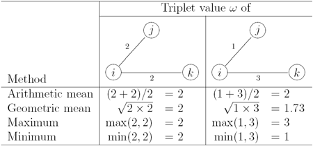
We can generalise the clustering coefficient, C, to take tie weights into consideration by rewriting Equation 2 and defining a triplet value, . It is vital to use an appropriate method for defining the value of a triplet as this impacts on the outcome of the coefficient. The method should be chosen based on the research question as well as the way in which the weights of the ties are operationalised. First, the triplet value, , can be defined as the arithmetic mean of the weights of the ties that make up the triplet. This is the simplest method of calculating the triplet value. However, this method is not sensitive to differences between the two tie weights as an extreme value can have a major impact on the triplet value. Second, can be defined as the geometric mean of the weights attached to the two ties. This method overcomes some of the sensitivity issues as the triplet made up by a tie with a low value and a tie with a high value will have a lower value than if the arithmetic mean were used. Additional methods defines the triplet value as the maximum or minimum value of the two weights. These two methods represent extreme cases. The “maximum” method offsets a low tie weight and makes a triplet with a strong tie and a weak tie equal to a triplet with two strong ties. Conversely, the “minimum” method offsets a high tie weight by making triplets with a strong tie and a weak tie equal to triplets with two weak ties. Table 1 highlights the differences between the methods of defining the triplet value. We will explore them further at the end of Section 2.3.

Once an appropriate method for defining has been chosen, we can generalise the clustering coefficient to take into account as follows (equation 3):

The generalised clustering coefficient produces the same result as the binary clustering coefficient if applied to a binary network. This is because all triplets have the same value, , irrespective of the method used to calculated triplet value. In addition, the generalised coefficient shares the same properties of the binary coefficient. It still ranges between zero and one because neither numerator nor denominator of the fraction can be negative; moreover, every element that can be part of the numerator is part of the denominator. In a completely connected, network all triplets are closed as the third tie will always be present, e.g. between node j and node k in Table 1. Therefore, all triplets are part of both the numerator and denominator: . To test whether as the size of a classical random network increases or, more specifically, equals the probability dyads to be tied together, we created a set of random networks with different sizes, but with a fixed degree. Since classical random networks are binary, we assigned a random weight between 1 and 10 to the ties in an effort to simulate a weighted network. We applied the generalised clustering coefficient to these networks, and found that as the network size increases. In particular, as shown by Table 2, we found that was very close to the probability of a tie in classical random networks. Furthermore, to assess the sensitivity to weights, we tested the generalised clustering coefficient on networks where the network structure was not randomised, but where the weights are randomly assigned to the ties. We found , where is the clustering coefficient calculated on binary networks where all ties with positive values are set to present.¹

Table 2: Simulations of the generalised clustering coefficient on ensembles of classical random networks with 50, 100, 200, 400, 800, and 1,600 nodes and an average degree of 10 where ties are assigned a random weight between 1 and 10. Each ensemble contains 1,000 scenarios. The four methods for defining triplet value were not significantly different (p>0.7).

In this chapter, we assume that weights are positive values and that a higher value is better than a lower one. In situations where the second part of this assumption is not appropriate, e.g. when weights of ties refer to costs and lower values are better than higher ones, weights should be inverted (Newman, 2001c). Then, in the example of costs, a low cost will have a higher value than a high cost. Furthermore, we will use the absolute values of weights without normalising them (e.g., by dividing them by their maximum or average) as this would have no effect on the results of our analysis.

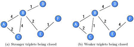
To illustrate and exemplify the applicability of the generalised clustering coefficient, Figure 2 shows two sample networks with six nodes and six weighted ties. In network a, the ties between the nodes that form the triangle have a higher weight than the average tie weight in the network, whereas the reverse is exemplified in network b.

Figure 2: Two weighted sample networks.

Both sample networks have the same binary clustering coefficient if the networks are transformed by setting ties with a weight greater than 0 () to present (equation 4):

However, we believe it is not accurate to claim that both these networks have the same tendency of “friends to be friends themselves” (Freeman, 1992). Friendship can be assessed using the same criteria that Granovetter (1973) used for defining tie weights (duration, emotional intensity, intimacy, and exchange of services). If, for example, the tie weights in the sample networks in Figure 2 correspond to duration, we can say that the nodes in network a are spending more time on other nodes that are themselves tied together than in network b. In turn, it could be argued that node B‘s friendships are transitive in network a, whereas the node’s acquaintances are transitive in network b.

The generalised clustering coefficient shows a difference between the two sample networks. For network a and b in Figure 2, the coefficients obtained by using the “geometric mean” method for defining the triplet values () are respectively (equations 5a and 5b):

The difference between the two coefficients results from the fact that the generalised clustering coefficient captures more information than the binary one. In fact, the difference between Equation 5a and 5b is a reflection of the differences in tie weights of the two sample networks. Burt (1992, 2005) defined a person as a less efficient information broker if he or she spends time with people that are themselves connected or part of the same group. Conversely, if the person spends time with disconnected people or people part of different groups, he or she could act as a gateway and control the information flowing between the people or groups. If the sample networks were knowledge networks, it can be argued that the people in network a are less efficient in being brokers and are in less advantageous positions to control information than the ones in network b.

The weight of the closing tie of a triplet is not considered in the proposed generalisation of the clustering coefficient. This is because we believe that the aim of the clustering coefficient is to assess the likelihood of the closing tie to be created, and not the strength of this tie. Formally, we see the closing tie as a product of the triplet. In other words, as networks evolve over time by the creation and removal of ties, clustering occurs when a triplet exists and a third tie is created, so that the triplet is closed. However, in a cross-sectional network, we only observe a triangle and cannot determine which of the three triplets, that make up the triangle, occurred first. In effect, this means that the weight of the closed tie of a triplet is considered since it is part of the other two triplets in the triangle. Chapter 4 extends the proposed generalised coefficient to weighted longitudinal networks.
_____________________
¹ This finding is based on the empirical networks presented in Section 2.3. For each network, we reshuffled the weights globally among the ties in the network, and calculated . This randomisation procedure maintains the topology of the observed network, and therefore does not change. We compared (1,000 scenarios) to C and found that they were not statistically significantly different.