Tore Opsahl

Thesis: 5.3 Longitudinal network functions

For longitudinal networks, the main function implemented in tnet is the method presented in Chapter 4. This function is called tnet.growth.clogit and probes the underlying mechanisms that guide nodes’ choices in where to direct their ties. This function is general and not limited to the analysis conducted in Chapter 4 or online communication data. The only requirement is that the data represents a directed network where the exact sequence in which ties were formed is known. The data can be both binary and weighted.

As outlined in Chapter 4, multiple mechanisms are thought to guide the formation of ties. These mechanisms are based on the network as well as information about the nodes. Each of these mechanisms can in turn be operationalised as a set terms or independent variables. These terms are given through a vector to the tnet.growth.clogit function — at least one term must be included. The network terms that are implemented are illustrated in Figure 20. Node i creates a tie to a possible target node h (the focal dyad, dashed line). The , , and nodes are the ones that node i is already tied to, and the , , , and nodes are the ones that node i is not tied to, but are already tied to h.

First, three terms are included to account for the increased likelihood of forming a tie if two nodes share common contacts (Heider, 1946). The basic term is the number of node i‘s contacts that are tied to node h. This term is named "triadic.closure". In the sample network in Figure 20, this term is equal to 2 for the focal dyad. However, as shown in Chapter 2, clustering can be generalised to weighted networks. This generalisation requires the use of a triplet value, which is based on the weights of the two ties that indirectly connect a node to another. Currently, the tnet.growth.clogit-function includes two triplet terms where the triplet values are based on the “minimum” ("triadic.closure.w.min"; equal to 5 in the example) and “geometric mean” ("triadic.closure.w.gm"; equal to 6.29 in the example) methods. These two methods are also illustrated by Figure 14a and b, respectively.

Second, two terms are included to measure the effects of popularity in networks (Dorogovtsev and Mendes, 2003). The first term is the in-degree of nodes. This term has simply been named "indegree". In this example, this would be equal to 6. In weighted networks, this term can be extended to the in-strength of a node, which is the sum of weights attached to the ties terminating a node ("instrength"; equal to 18 in this example).

Third, terms are included to test reciprocity (Gouldner, 1960; Plickert et al., 2007). The simplest is a dummy term that is equal to 1 if a tie exists from node h to node i, and 0 otherwise ("reciprocity"). This term can also be extended to weighted networks to the weight of the tie from node h to node i ("reciprocityw"). Since a tie is present from node h to node i with a weight of 3 in the example, these terms would be equal to 1 and 3, respectively.

Fourth, ties can be reinforced in weighted networks (Krackhardt, 1992). Therefore, the weight of the tie from node i to node h can be included ("reinforcement") to account for the increase in likelihood of directing a tie towards another node that already have been contacted. In the example, this would be equal to 2.

Moreover, the effect of node similarity by sharing or having a similar node attribute on the likelihood of forming a tie can be included through the inclusion of demographic (homophily) or positional (focus constraints) attributes. The node attribute must be transformed into dyadic terms. Two methods have been programmed in tnet.growth.clogit-function to do this process. The first method is to create a dummy term that is equal to 1 if the two nodes have the same value of the attribute, and 0 otherwise. This method can be used for both nominal and ordinal attributes. The second method is specifically designed for ordinal attributes. It takes 1 minus the standardised difference between the values of the attributes for the two nodes. For example, if people’s age is known in a social network of 30 to 40 year-old individuals, then the first term would be equal to 1 if two people (i and h) were of the same age (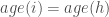), whereas the second term would be equal to: . Terms based on these two methods are included by loading the node attribute as separate vectors in the R-session, and adding the name of these vectors prefixed with same. or simi. to the list of terms, respectively. For example, if the age of the people is loaded as a vector named ageofperson, the term to study the effect of similar age on the likelihood of a tie being formed would be "simi.ageofperson".

However, if these two methods are not sufficient for creating a dyadic term, then the tnet.growth.clogit-function also allows for the inclusion of a user-created matrix where a dyad term is explicitly defined. This should be an matrix with, for example, the log of the number of miles separating two nodes (e.g. Sorenson and Stuart, 2001). If this matrix was named logmiles, then "dyad.logmiles" should be added to the list of terms to study the impact of geographical closeness on tie formation.

The tnet.growth.clogit-function can easily be extended by the inclusion of additional terms (or independent variables). The simplest way to do this is to output a table with all the observations and variables instead of the results from a regression (This is done by setting the switch regression to FALSE.). Then the researcher can add variables to this table, and then run a regression in either R or other statistical programmes (The clogit command in Stata is able to run a conditional logistic regression (StataCorp, 2007). The easiest way to export the regression table from R to Stata is to use the foreign-package’s write.dta function, e.g. write.dta(output, file="c:/statafile.dta"), where output is the regression table and c:/statafile.dta is the location of the file.). For example, if interaction terms are to be included, this can easily be done using this method. Moreover, a researcher with basic knowledge of R programming can also alter the source code. Each term is coded as a module and additional modules can easily be inserted in the code. The supporting website contains the specific details for inserting user-created modules.

In addition to the tnet.growth.clogit-function, tnet also includes a function to randomise a longitudinal network, rg.longitudinal. This function is flexible and allows the random network to be constrained in a number of ways. First, either creator or target nodes can be maintained. This guarantees that the out-degree or in-degree distributions are maintained at every t. Second, it can keep the size of the network invariant by maintaining either the available nodes in the network (regardless of whether they are connected) or the number of connected nodes at every t. Third, it can maintain the weight distribution at every t. It does so by finding the duplication of ties (reinforced ties) in the network, and replicating a randomised tie when the observed tie was reinforced. For example, if a tie is formed between two nodes at and reinforced again at in the observed network, then the tie at is randomised and the tie at is equal to the randomised one at .