Tore Opsahl

Random Networks

When analysing network and computing measures, it is difficult to gauge whether the outcome is “high” or “low”. For example, is a clustering coefficient of 0.3 high or low? Random networks based on an observed network can be used as to create a benchmark value. In other words, an observed value (e.g., a clustering coefficient) can be compared to the distribution of clustering coefficient from corresponding random networks.

There are many procedures or null models for creating random networks. These procedures vary in how much they randomise an observed network. Traditionally, classical (also known as Bernoulli or Erdos-Reyni) random networks were the commonly used. These networks are constructed by using the same number of nodes, and assigning each dyad a uniform probability of having a tie based on the number of observed ties. In these networks, the degree distribution is uniform or Poisson. However, such a distribution rarely exist in reality. In fact, most real-world distributions are skewed.

In response to the lack of comparability between observed networks and classical random networks, a set of randomisation procedures that maintain additional features has been developed. First, by reshuffling ties in an observed network, it is possible to create random networks that maintain each node’s number of ties as well as the overall number of nodes and ties (Molloy and Reed, 1995). Second, for weighted networks, it is also possible to reshuffle only the weights. By maintaining the ties and simply reshuffling tie weights, features based on connectedness are maintained (e.g., the size of the largest interconnected group of nodes; Opsahl et al., 2008).

Classical Random Networks

Classical random networks are created by setting the number of nodes and giving all possible ties a uniform probability of being formed. Given that each tie is independent of all other ties, it is often possible to approximate the value of a measure mathematically without the need of simulations when using these networks. For example, the global clustering coefficient is equal to the uniform probability and the average shortest path is approximately the ratio between the logarithm of nodes and the logarithm of the average number of ties that nodes have (Watts and Strogatz, 1998). A main limitation of classical random networks is that the distribution of ties across nodes is uniform or Poisson. While this in convinient for deriving expected values, such a distribution rarely exist in reality. In fact, most real-world degree distributions are skewed, which implies that a few nodes are hubs. The hubs particulily affect network measures based on shortest paths as hubs reducing it by acting as shortcuts among other nodes.

Link Reshuffling

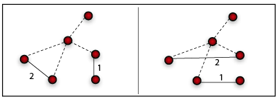
As nodes’ degree are not uniformely distributed, a second procedure for creating random networks consists in reshuffling the topology, reaching the maximally random network with the same degree distribution as the observed network (Maslov and Sneppen, 2002; Newman, 2003). It does so by randomly selecting two ties, and . The two ties are then rewired by setting and . The weights are automatically redistributed by remaining attached to the reshuffled ties. However, if either of these ties is already formed, this step is reverted, and two new ties are selected. This condition guarantees that multiple ties are not formed between two nodes, which ensures that the weight and degree distributions remain unchanged. If this procedure is repeated enough times, the outcome is a corresponding random network. This model is commonly used in the Physics literature; however, each of the random networks that are produced is not produced with an equal probability. For more details, see Snijders (2001) and Rao et al. (1996).

One step of the link reshuffling procedure for an undirected netwok. Note that while a node maintain its out-strength in a directed network, this is not the case in an undirected network.

Weight Reshuffling

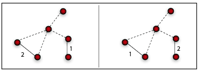
While the link reshuffling procedure can be applied to binary networks, two other procedures are possible to use when dealing with weighted networks. The weight reshuffling procedure consists simply in reshuffling the weights globally in the network (Opsahl et al., 2008). This null model maintains the topology of the observed network. Therefore, the number of ties originating from a node (degree) does not change. Moreover, other features, such as the giant component does not change as well.

One step of the weight reshuffling procedure for an undirected netwok

Local Weight Reshuffling

Inevitably, since weights are reshuffled globally using the link and weight reshuffling procedures, they produce random networks in which the nodes do not maintain the same node strength as in the observed network. Local weight reshuffling is a third randomisation procedure for directed networks that preserves this quantity by reshuffling weights locally for each node across its outgoing ties (Opsahl et al., 2008). The procedure can be extended to undirected networks by duplicating an undirected tie into two directed ties – one in each direction. It should be noted that this procedure breaks the weight symmetry in the two directions of an undirected tie (the topology remains invariant). The appropriateness of this method for undirected networks depends on the research setting and how tie weights are defined. For example, its applicability to undirected transportation networks is justified by the typically directed nature of traffic flows (although the US airport network displays a high symmetry; Barrat et al., 2004).

One step of the local weight reshuffling procedure for a directed netwok

Example

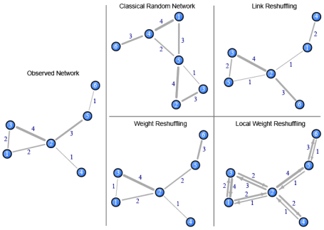
To highlight how the various procedures differ, the diagram below shows an observed network and the four random networks introduced above. To reproduce these networks, see the R code below.

Random networks created using the null models outlined above. The classical random network uses the same number of nodes, a 0.4 uniform probability of ties being present, and tie weights randomly picked between 1 and 4.

Want to test it with your data?

The randomisation procedures are implemented in tnet. First, you need to download and install tnet in R. Then, you need to create an edgelist of your network (see data structures in tnet for weighted one-mode networks). The commands below show how the edgelist for the sample network here can manually be entered, and how to apply the randomisation procedures.

# Load tnet
library(tnet)

# Create a Classical Random Network with 6 nodes and a 0.4 uniform probability of ties being created
rg_w(nodes = 6, arcs = 0.4, weights = 1:4, directed = FALSE)

# Load an observed network
net  <- cbind(
i=c(1,1,2,2,2,2,3,3,4,5,5,6),
j=c(2,3,1,3,4,5,1,2,2,2,6,5),
w=c(2,2,2,4,1,3,2,4,1,3,1,1))

# Link reshuffling of the sample network
rg_reshuffling_w(net, option="links")

# Weight reshuffling of the sample network
rg_reshuffling_w(net, option="weights")

# Local weight reshuffling of the sample network
rg_reshuffling_w(net, option="weights.local")

To recreate the illustration of the random networks, the code below is the first step. The diagram above was made a bit nicer afterwards using Adobe Illustrator.

# Load tnet and the observed network
library(tnet)
net  <- cbind(
i=c(1,1,2,2,2,2,3,3,4,5,5,6),
j=c(2,3,1,3,4,5,1,2,2,2,6,5),
w=c(2,2,2,4,1,3,2,4,1,3,1,1))

# Create object to hold the random networks
rn <- list()

# Put the four random networks in the object (using seed=1 for replication purposes)
rn[[1]] <- rg_w(nodes = 6, arcs = 0.4, weights = 1:4, directed = FALSE, seed = 1)
rn[[2]] <- rg_reshuffling_w(net, option="links", seed=1)
rn[[3]] <- rg_reshuffling_w(net, option="weights", seed=1)
rn[[4]] <- rg_reshuffling_w(net, option="weights.local", seed=1)

# Convert networks to igraph format
net <- tnet_igraph(net)
rn <- lapply(rn, function(a) tnet_igraph(a))

# Set up plot
par(mfrow=c(2,3), pty="m", mar=c(4,5,0.1,0.1), xaxs="r", yaxs="i")

# Get layout of observed network
layout <- layout.fruchterman.reingold(net)

# Plot observed network
plot(net, main="Observed Network", layout=layout, vertex.label=1:6, edge.width=E(net)$weight, edge.label=E(net)$weight)

# Plot random networks
plot(rn[[1]], main="Classical Random Network", layout=layout.fruchterman.reingold, vertex.label=1:6, edge.width=E(rn[[1]])$weight, edge.label=E(rn[[1]])$weight)
plot(rn[[2]], main="Link Reshuffling", layout=layout.fruchterman.reingold, vertex.label=1:6, edge.width=E(rn[[2]])$weight, edge.label=E(rn[[2]])$weight)
plot.new()
plot(rn[[3]], main="Weight Reshuffling", layout=layout, vertex.label=1:6, edge.width=E(rn[[3]])$weight, edge.label=E(rn[[3]])$weight)
plot(rn[[4]], main="Local Weight Reshuffling", layout=layout, vertex.label=1:6, edge.width=E(rn[[4]])$weight, edge.label=E(rn[[4]])$weight, edge.arrow.size=0.5)

References

Barrat, A., Barthelemy, M., Pastor-Satorras, R., Vespignani, A., 2004. The architecture of complex weighted networks. Proceedings of the National Academy of Sciences 101 (11), 3747-3752. arXiv:cond-mat/0311416

Molloy, M., Reed, B., 1995. A critical point for random graphs with a given degree sequence. Random Structures and Algorithms 6, 161-180.

Opsahl, T., Colizza, V., Panzarasa, P., Ramasco, J. J., 2008. Prominence and control: The weighted rich-club effect. Physical Review Letters 101 (168702). arXiv:0804.0417.

Watts, D. J., Strogatz, S. H., 1998. Collective dynamics of “small-world” networks. Nature 393, 440-442.